- Clustering vs. classification
- Unsupervised learning
- Applications
- Measures of (dis-)similarity
2021-11-15
Introduction
Classification
Classification can be observed as sorting of objects into a predefined classes
- defined model (classification rules)
- “predicts” discrete classes
- supervised learning
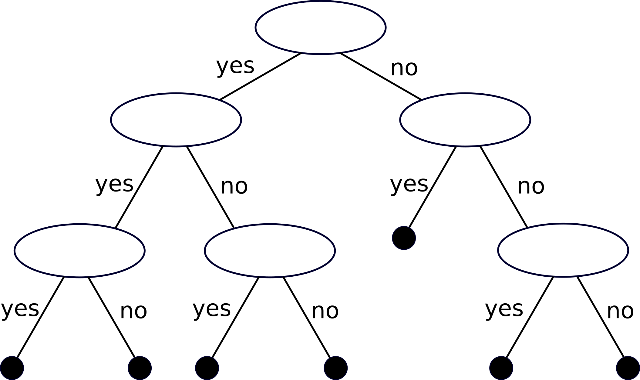
Classification tree.
Clustering vs. classification
Main task of clustering - as opposed to classification - is to identify smaller groups (clusters) within a larger set.
- exploratory and explanatory
- description, not a model
- usually not utilized for prediction
- unsupervised learning
Supervised vs. unsupervised learning
Scholars usually classify (N.B. not cluster!) learning algorithms into a two categories (or classes, but not clusters) - supervised and unsupervised.
Two classes, because there is a predefined notion on their difference - whether one uses the information from a supervisor or not.
Supervisor - predefined authority.
Can we trust it?
In certain use cases one is allowed to question supervisor
- a cat with moustaches
Who classified the learning algorithms into a two categories in the first place? Why not three or four?
- semi-supervised learning and reinforced learning
N.B. Whatever algorithm classification you use, remember that this is ALGORITHM classification, not a PROBLEM classification. Sometimes YOU define problem (e.g. a cat with moustaches).
Applications of clustering
- Understanding
- e.g. find similar documents, or documents written by the same person
- e.g. find set of genes or proteins that act together
- Summarization
- e.g. reduce the set size or the dimensionality of the problem
Clustering
Clustering main task is to identify smaller groups (clusters) within a larger set so that:
- Objects within a cluster should be similar (or related)
- …that can be measured with intra-cluster similarity measure
- Mutual clusters should be different (or unconnected)
- …that can be measured with inter-cluster similarity measure
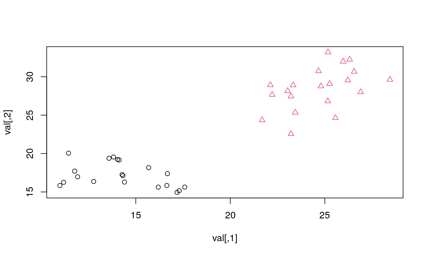
Let’s visualize that…

Different clusters within initial set.
Object similarity
There are multiple approaches to define similarity between objects:
- an entropy measure to measure homogeneity of a cluster
… or measure similarity based on how two objects are related to one another, e.g.
- correlation
… or some distance measure in selected feature space
- Euclidean distance
- Manhattan (taxicab) distance
- Mahalanobis distance
- various \(L^p\) norm
Intra- and Inter-cluster similarity
Intra-cluster similarity (distance)
- Measures distance between object within a single cluster
- As the simplest example the distance between object can be used
Iner-cluster similarity (distance)
- Measures distance between clusters
- As the simplest example the distance between two cluster centers can be used
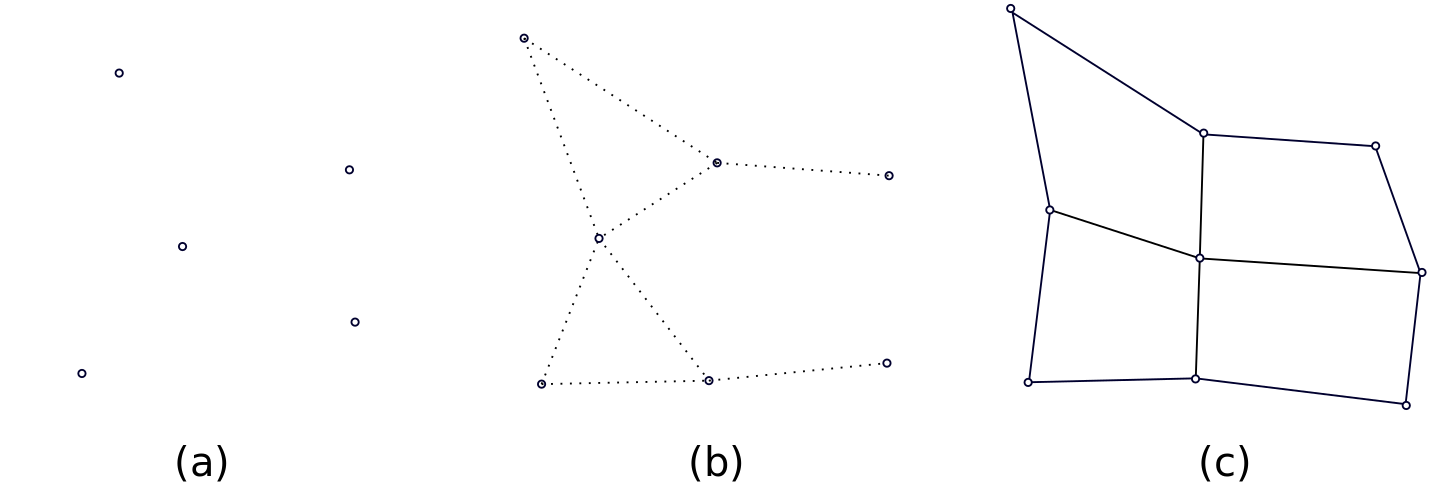
Cluster
- Why the notion of cluster is not well defined?
- Examples
- Some properties of a cluster
Why the notion of cluster is not well defined?
Similarity, proximity and cluster is in the eye of the beholder.
Sometimes it is not simple to unambiguously define the number of clusters or whether an element belongs to a cluster A, or a cluster B.
Let us observe few examples and ask ourselves where should we put the border between the clusters?
How many clusters do you see?

Two, right?
…err, I mean four…
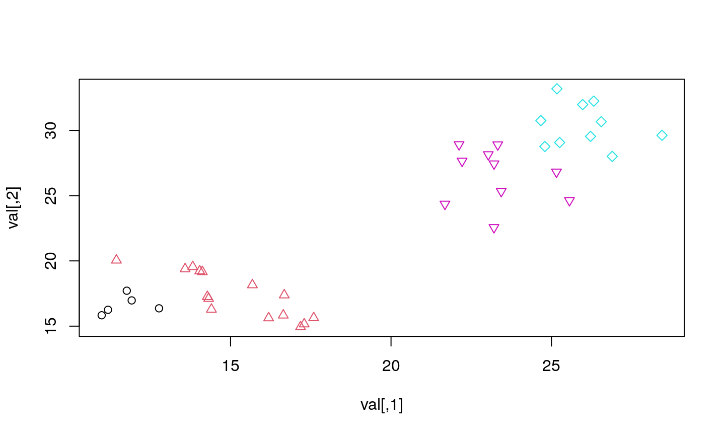
…actually, yes, four…

…how sure are we for these elements?
Actually…

…the elements in this dataset came from 8 (eight!) different distributions…
This is not just a statistical problem!
This is not just a machine problem.
And things get even more complicate when we try to transfer the human knowledge (or perception) to machines.
How many faces do you see?

How many horses do you see?

Instead of conclusion
Clustering is hard and may provide multiple solutions. From these solution we cannot a priori select the good ones.
Elements may belong to class A or B, and sometimes to both of them. Do the clusters overlap is not always easy to conclude from the available data.
We can come to different solutions, based on the certain assumptions (sometimes made implicitly) not related to data.
Cluster properties and some clustering algorithms
- Properties
- Examples
- Algorithms
Some properties of a cluster
- Non-overlapping
- Centered
- Proximity (between elements)
- Distribution density
- Known cluster shape
The correct approach for clustering algorithm selection would be to first contemplate on the properties of a cluster that we may assume.
The accuracy of the clustering algorithm depends on how accurate these assumptions are.
…for example
- Partitional clustering
- divides the set into mutually non-overlapping subsets
- Hierarchical clustering
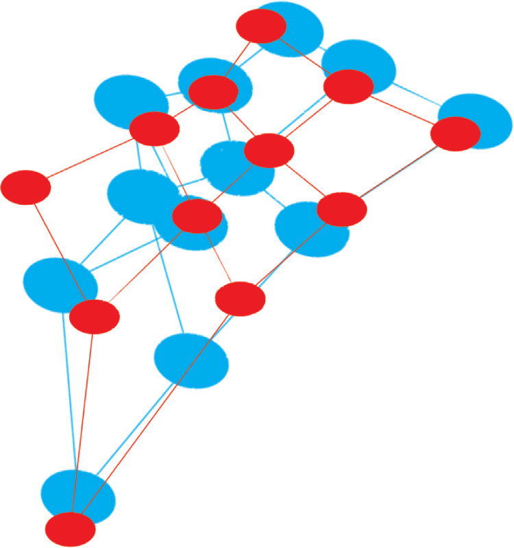
- An object belongs to a set of mutually nested subsets
- Nesting can be visualised with a hierarchical tree or dendrogram
Partitional clustering

Hierarchical clustering

Clustering algorithms examples
Some of the well known and often used algorithms for clustering fall into one of the following category:
- K-centers family algorithms
- Hierarchical clustering
- Density-based clustering
k-centers algortihm
- Partitional clustering algorithm that split initial set into several (non-overlapping) sets
- Each cluster has its “center”
- Each element is assigned to a group whose center is the closest
- Number of clusters must be known in advance
If as a “center” of the algorithm we use the mean value (centroid), the algorithm is know as a k-centers or k-centroids.
If as a “center” we use the median value (medoid) the algorithm is known as k-medoids.
The algorithm
- Select initial K centers
- Repeat…
- Partition the set into K clusters by assigning the elements to cluster whose center is the closest
- Calculate the cluster centers and adapt K centers towards them
- …until centers “move”
Algorithm properties
- Simple
- The original algorithm randomly selects the initial location for cluster centers
- Different initialization might produce different results
- Data point proximity to center can be calculated with a simple similarity metric:
- Euclidean distance, cosine similarity, correlation…
- Algorithm converges
- Fast
- Locally
Disadvantages
- Sensitivity to initial cluster center selection
- Poor choice might provide poor results
- Typically, algorithm might not provide good results if:
- Clusters are not of the same size
- Clusters do not have the same density
- Clusters do not have spherical shape
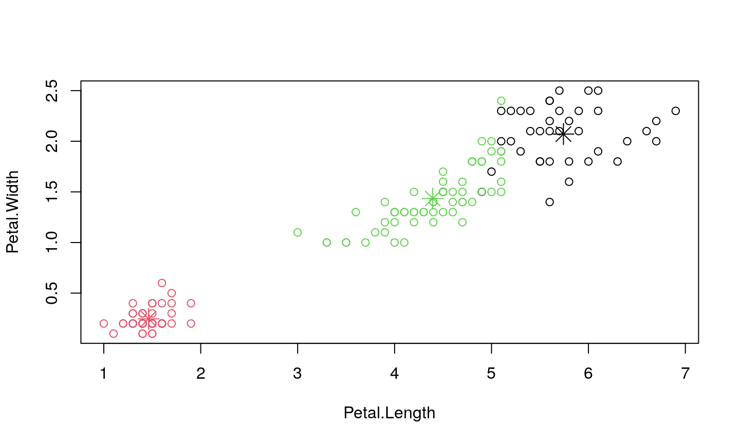
Example (Iris dataset)
Iris dataset - 150 items, 3 species, 50 instance of each - 4D space - petalum and sepalum width and height - can we identify the number of species and differentiate between them
Results
Centers:
##   Sepal.Length Sepal.Width Petal.Length Petal.Width
## 1     6.850000    3.073684     5.742105    2.071053
## 2     5.006000    3.428000     1.462000    0.246000
## 3     5.901613    2.748387     4.393548    1.433871
To which cluster is each element assigned:
##   [1] 2 2 2 2 2 2 2 2 2 2 2 2 2 2 2 2 2 2 2 2 2 2 2 2 2 2 2 2 2 2 2 2 2 2 2 2 2
##  [38] 2 2 2 2 2 2 2 2 2 2 2 2 2 3 3 1 3 3 3 3 3 3 3 3 3 3 3 3 3 3 3 3 3 3 3 3 3
##  [75] 3 3 3 1 3 3 3 3 3 3 3 3 3 3 3 3 3 3 3 3 3 3 3 3 3 3 1 3 1 1 1 1 3 1 1 1 1
## [112] 1 1 3 3 1 1 1 1 3 1 3 1 3 1 1 3 3 1 1 1 1 1 3 1 1 1 1 3 1 1 1 3 1 1 1 3 1
## [149] 1 3
Number of elements in each cluster:
## [1] 38 50 62
Confusion matrix
Confusion matrix is usually utilized to measure classification accuracy.
Confusion matrix is an intuitve way to show how correctly do we assign each element to a certain cluster (or class):
table(iris$Species, kc$cluster)
##
##               1  2  3
##   setosa      0 50  0
##   versicolor  2  0 48
##   virginica  36  0 14
Visualization
Let’s visualize the results.
Note that he problem is 4D in nature since there are 4 features.
Therefore, we will visualize this in two 2D panels.

Conclusion
From the figures, one might conclude that the results are inaccurate, as some points are obviously closer to the center of some other cluster. Actually, we simply get that impression since we observe the projection of 4D problem to 2D, so the distance between data points and a cluster center is distorted.
Perhaps the following animation would convince you that the coloring is right.
Hierarchical clustering
- Advantages
- Various types
- Example
Advantages
- It is not necessary to know the number of clusters in advance
- As we will seen, this can be decided later on
- Can be used to identify the number of clusters for some other algorithm
- Hierarchical clustering might reflect the true taxonomy
- e.g. in biology
Types of hierarchical clustering
- Top-down approach or Divisive hierarchical clustering
- Starts with one cluster that contains all the elements
- Recursively splits clusters into sub-clusters until it each cluster contains one element
- Splitting can be stopped when a predefined number of clusters is reached
- Bottom-up approach or Agglomerative hierarchical clustering
- Starts with the each element as separate cluster
- Merges clusters until there is only one cluster
- Merging can be stopped earlier when a predefined number of clusters is reached
A sketch of the algorithm
- Use the similarity or proximity matrix
- Split or merge elements of the matrix…
- … and recalculate the similarity matrix
The most notable difference between various algorithms is a similarity/proximity measure
Some examples of cluster proximity measure
- Minimal distance (distance between two closest elements)
- Maximal distance (distance between two farthest elements)
- Mean (or median) distance of each pair of elements
- Distance between cluster center (calculated as e.g. mean)
- Squared error (or minimum variance criterion, or Ward’s method)
Agglomerative hierarchical clustering
Let’s demonstrate it on our Iris dataset once again.
For illustration, only few dozens of elements will be observed.


N.B.
We do not know the true labels of the elements.
By performing clustering we again get the only the abstract labels, same as earlier:
##   1   2   3   4   5   6   7   8   9  10  51  52  53  54  55  56  57  58  59  60
##   1   1   1   1   1   1   1   1   1   1   2   2   2   3   2   3   2   3   2   3
## 101 102 103 104 105 106 107 108 109 110
##   4   4   4   4   4   4   3   4   4   4
Divisive hierarchical clustering
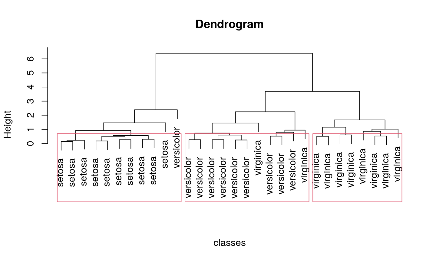
Conclusion
On the same dataset, the top-down approach provided better slightly different results.
This is just an example.
Density clustering
- Motivation
- DBSCAN algortihm
- Advantages and disadvantages
- Example
Motivation
Sometimes we cannot assume the shape of the cluster or even know that any assumption on the cluster shape is void. Under certain circumstances, the cluster center (if calculated as a center of gravity) might event not be the element of a cluster.
In order to cope with this type of a problem we have to utilize other cluster properties.
Human perception clusters elements not only according to proximity, but according to density as well. This is what motivates the density based clustering.
An example
Imagine you have object like the one shown in the bottom figure…
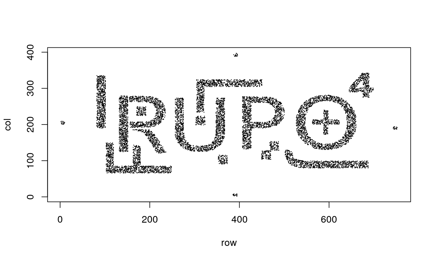
… you will simply identify them as letters or numbers, right?
A noisy example
Even if we add noise to our problem - we can still identify the elements.

However, none of the previous algorithms would perform well in this case…
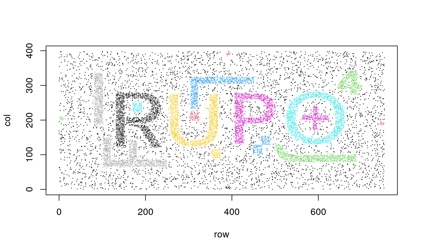
DBSCAN algorithm
Density-based spatial clustering of applications with noise (DBSCAN) algorithm is an algorithm that provides decent results for these type of problems.
DBSCAN algorithm is more than 20 years old and since 2014 it belongs to algorithms with “test of time award”.
Algorithm basics
- Define density as a number of points in a given radius (parameter
eps) - Identify three type of points using following definitions:
- Core point
- each point that has more then a minimal number of points (parameter \(m\)) in a given radius
- Border point
- each point that does not have the minimal number of points within a given radius, but have at least one core point
- Noise
- points that are neither core, nor border points
- Core point
The algorithm
- Remove noise
- Fore each core point
- If it is not associated with any cluster associate to a new cluster
- Each point in the neighborhood (as defined by
eps) of that cluster- if it is not associated to any other cluster associate to this one
Advantages
DBSCAN algorithm:
- Does not need to know the number of clusters
- Can identify clusters of arbitrary shape
Works even when the excessive noise is present and is resilient to outliers
Requires only two parameters to tune
Disadvantages
- DBSCAN is not fully deterministic algorithm
- Border points might belong to different clusters if different implementation process the data in different order
- However, it is deterministic for core points and noise
- The usability of the algorithm depends on the distance metric used
- Typically this is Euclidean distance which is useless in high dimensional problems due to the curse of dimensionality
- DBSCAN does not perform well if there are multiple clusters with significantly different densities
Clustering results
Clustering as a dimensionality reduction
- Dimensionality reduction
- Self-organising maps
- (Growing) Neural gas
- Manifold learning
- Examples
Dimensionality reduction
Clustering is explanatory technique and can be observed as a dimensionality reduction technique.
We are using just few data to describe the whole dataset - we reduced the amount of information necessary to describe the dataset.
Now, if we have more information on the relationship between data, we could describe data not just as “blobs” (clusters).
SOM and GNG
Self-organising maps (SOM) and (Growing) Neural gas (GNG) provide such an opportunity. If they are used as a clustering algorithms they will use the the distance information (neighborhood) to describe the data.
Due to this additional information the cluster may not have a predefined shape, but their (predefined) relationship will be contained in the neighborhood structure.
This structure is referred to as lattice. SOM has a rigid lattice structure, while (G)NG has more loose lattice structure.
Lattice structure of: (a) SOM and (b) GNG. K-means (c) has no lattice structure.
Alignment of the lattice structure
Kalinić et al. “Sensitivity of Self-Organizing Map surface current patterns to the use of radial vs. Cartesian input vectors measured by high-frequency radars”, Computers & Geosciences, 2015

Vilibić et al. “Self-Organizing Maps-based ocean currents forecasting system”, Scientific Reports, 2016
Matić et al. “Adriatic-Ionian air temperature and precipitation patterns derived from self-organizing maps: relation to hemispheric indices”, Climate Research, 2019
Manifold learning
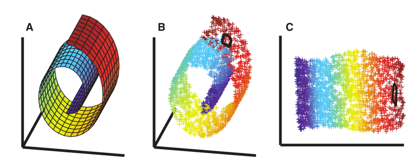
Roweis and Saul “Nonlinear Dimensionality Reduction by Locally Linear Embedding”, Science, 2000
Intro to neural networks
- Artificial neural networks
- Properties
- Model of a neuron
- Activation function
- Network architecture
Neural networks
Biological and artificial
ANNs:
- historically inspired by a biological model
- very simplified model
- implemented on a digital computer
Aims at:
- complexity
- parallel information processing
Artificial neural networks
- Perceptron
- Associative memory
- Multilayer perceptron (feedforward network)
- RBF neural network
- Recursive neural network
- Self-organising maps
- …
- Deep NN (including: LSTM, GAN, AE…)
Properties
- Nonlinearity
- Adaptability
- Supervised learning
- Scalability
- Neuro-biological analogy
Model of a neuron
There are three main part of a neuron model:
- Nonlinear activation function
- Summation
- Synapses
Each synapse \(j\) is represented as a wight \(w_j\) that multiplies input signal \(x_j\) before summation.
After summation the activation function \(\psi\) transforms the signal to output (usually denoted as \(y\)).
In case of classification the activation function typically limits the output to range \([0,1]\).
Graphical representation of a model
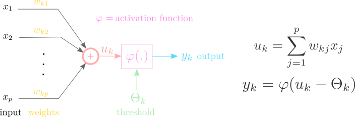
Activation function often has another parameter denoted as \(\Theta\) - which can be interpreted as a threshold.
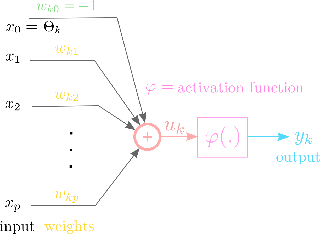
As an alternative, threshold can be implemented as an additional input \(x_0 = -1\), with weight \(w_0=\Theta\).
Activation function
Typical activation (transfer) function used in neural networks:
- Heaviside step function
- Piecewise linear function
- Sigmoid (sigmoidal, s-shaped, logistic, hyperbolic) function
- ReLu (Ramp)
Heaviside
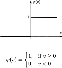
Heaviside activation function.
Piecewise linear
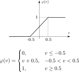
Piecewise linear activation function.
Sigmoid
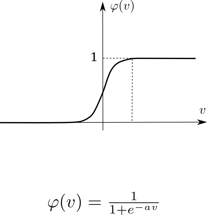
Sigmoid activation function.
Sigmoid activation function is a s-shaped function of a form:
\[ S(v)=\frac {1}{1+e^{-v}}, \]
which is a special case of a logistic function:
\[ f(v)=\frac {L}{1+{\mathrm e}^{{-k(v-\Theta)}}} \]
where \(k\) defines slop, and \(L\) the maximal value a function can achieve.
Logistic function relates to hyperbolic tangens \(tanh()\):
\[ 2\,f(v)=1+\tanh ({\frac {v}{2}} ) \]
Therefore, the same activation function can be found under different names, but beware these names do tno necessary reflect how the activation function is implemented.
\[ \psi(v) = \frac {1}{1+e^{-av}}\]
ReLu
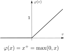
ReLu activation function.
Rectifier linear unit (ReLu), earlier know simply as “ramp” function. Is usually used in DNNs.
One smooth approximation to the rectifier is the “softplus” analytic function:
\[ f(v)=\ln(1+e^{v}) \]
Please notice the similarities to sigmoid function that can be observed as a smooth approximation of Heaviside step function.
Graphs
A (model of a) neural network is built from multiple neurons and their connections. This can be presented in a form of a directed graph where direction denotes the signal flow.
Two basic elements of such a graph are:
- synapse - input-output connection alongside its weight (edge)
- function - integrator alongside activation function (node)
Neural network architecture
Architecture or topology denotes how neurons (nodes) are mutually connected.
Basic topologies are:
- one-layer network
- multilayer network
- recurrent network
Naturally, recurrent network can also contain one or more layers
Multilayer networks
Recently, we distinguish between a shallow (classical) neural network and a deep neural network (DNN).
As a guideline we can consider a neural networks that require less feature engineering as a deep one.
Perhaps the most distinguishable DNN architectures that do not fall into a category of recurrent networks are information filtering networks and generative networks.
Perceptron
- How learning algoritm works?
- Simple model - one neuron
- Optimization
- Steepest descent
- LMS algorithm
ADALINE (a bit of history)
ADALINE - ADAptive LINear Element, is a model of the form:
\[ y_{i}=wx_{i}+\Theta \]
Notice that activation function is linear:
\[ \psi(x) = x \]
Now, assume we have \(N\) ordered pairs \((x_i, d_i)\) where \(d_i\) denotes the desired output for a given input \(x_i\).
Let us also assume that the relationship between \(x_i\) and \(d_i\) is approximately linear, i.e. the dots are (approximately) lie on a line.
If the line intersects with the origin (for simplicity) we can write:
\[d_i \approx w \cdot x_i \]
Learning as an optimization problem
The error made by this approximation can be expressed as:
\[ \varepsilon = d_i - w \cdot x_i \]
Now, ADALINE learning can be formulate as a search for a weight \(w\) for which the (absolute) error is minimal.
Absolute error is not differentiable therefore one usually use quadratic error \(\varepsilon^2\), or sum of squares (across all \(N\) pairs):
\[ J = \sum_{i=1}^N \varepsilon_i^2 = \sum_{i=1}^N (d_i - w \cdot x_i)^2\]
Analytical solution
This optimization problem has an analytical solution. The analytical solution can be found by looking where a partial derivative of \(J\) equals \(0\):
\[ \frac {\partial J} {\partial w} = 0\]
\[ \frac {\partial \sum_{i=1}^N (d_i - w \cdot x_i)^2} {\partial w} = 0\]
\[ -2 \, \frac {1} {N} \sum_{i=1}^N (d_i - w \cdot x_i) \cdot x_i = 0\]
The constant \(-2/N\) plays no significant role in our case, and we can make the following simplification:
\[ \sum_{i=1}^N d_i \cdot x_i - w \sum_{i=1}^N \cdot x_i^2 = 0 \]
\[ w = \frac {\sum_{i=1}^N d_i \cdot x_i} {\sum_{i=1}^N \cdot x_i^2} \]
Potential problems
Sometimes, the analytical solution is not the best option:
- It can be computationaly expensive (in terms of memory or time)
- Matrix operation (such as inverse) can cause numerical errors
- We wish to be able to adapt the results as we obtain more data
- It does not generalize well (e.g. if we change the activation function)
- …
Whatever the case might me, we can utilize an iterative procedure to find the minimum error - the gradient descent.
Gradient descent
Gradient descent uses the gradient information to find the local minumum of a given function. In order to do that it makes incremental steps in the direction opposite to (estimated) gradient at that location.
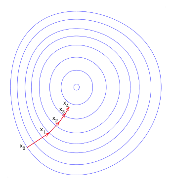
Gradient descent. Vectors shows adaptation step
In our case, we can calculate the gradient as follows::
\[ \nabla J = \frac {\partial J} {\partial w} = \frac {\partial} {\partial w} \left( \frac{1}{N} \sum_{i=1}^N \varepsilon_i^2 \right)= \frac{2}{N} \sum_{i=1}^N \varepsilon_i \frac {\partial } {\partial w} \varepsilon_i\]
Since the error is given by \(\varepsilon = d_i - w \cdot x_i\), after derivating by \(w\) we may express gradient as:
\[ \nabla J = -\frac{2}{N} \sum_{i=1}^N \varepsilon_i x_i\]
N.B.!
Was this useful?
- in order to calculate the gradient \(\nabla J\) we need to have all valuse of both \(x_i\) and \(\varepsilon_i\).
- if we can calculate the gradient in this way, we could calculate the analytical solution as well
However, sometimes we wish learing (weight adaptation) to be in real time, i.e. that neurons adapt as soon as ti gets a single datum, not the whole data set.
In order to achieve this, we use a gradient estimate. This estimate is no longer average value of the product \(\varepsilon_i \cdot x_i\), but the estimate is done with each new data sample, where we pick “a bit” of \(\varepsilon_i \cdot x_i\). We refer to this “bit” as a learning step, denote it by \(\eta\), and write:
\[ \nabla J \approx -\eta \cdot \varepsilon_i \cdot x_i\]
Thanks to this idea the research in the field of adaptation and learning machines started, where we distinguish on-line learning (as in previous example) where we learn on each sample, and batch learning were we adapt based on several samples at once.
Earlier this problem was always reduced to question why learn (sample-by-sample) if I can conclude (analytically) once I have all the data.
The problem of not having “all the data” was purely technical one.
Weight adaptation
With each new sample, the analytical problem has to be solved from the start, and this becomes more and more demanding (there is more and more data).
Therefore, we formulate the learning problem as a weight adaptation problem, and we know that this adaptation should go in the direction opposite to a gradient:
\[ w(k+1) = w(k) - \nabla J (k),\]
where \(k\) denotes a (discrete) time step.
LMS algorithm
- a learning rule, also known as Hebbian learning
- present in many adaptive systems
\[ w(k+1) = w(k) - \eta \cdot \varepsilon(k) \cdot x(k),\]
where \(k=i\) if time step corresponds to index of a new data sample.
Examples
- LMS algorithm implementation
- Batch learning
- On-line learning
- Convergence problem
LMS algorithm implementation
LMS algorithm can be easily implemented, either in the form of batch learning:
\[ w(k+1) = w(k) - \eta \sum_{i=1}^N \varepsilon_i x_i, \]
or on-line learning:
\[ w(k+1) = w(k) - \eta \cdot \varepsilon(k) \cdot x(k).\]
Excercise
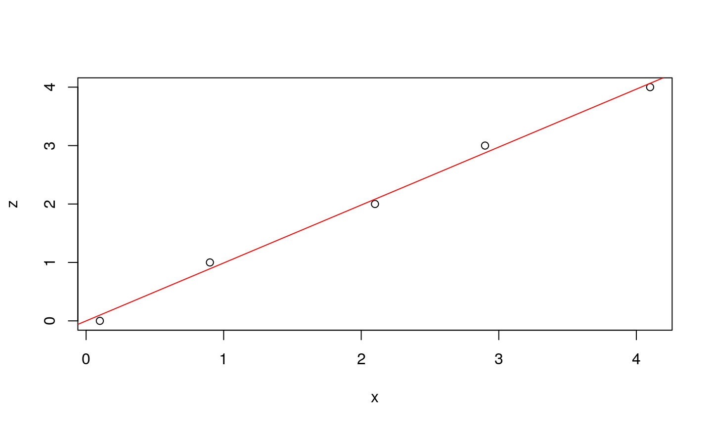
Let’s assume that we have a function given in the form of a look-up table. We know the desired values \(d_i\), while the parameters (\(x_i\)) are measured (terefore may contain noise). If the data are pairs (0.1,0),(0.9,1),(2.1,2),(2.9,3) i (4.1,4), one can visualize them on 2-D plane, alongside the line that represents the analytical solution.
Observe how weight adapts with each step…
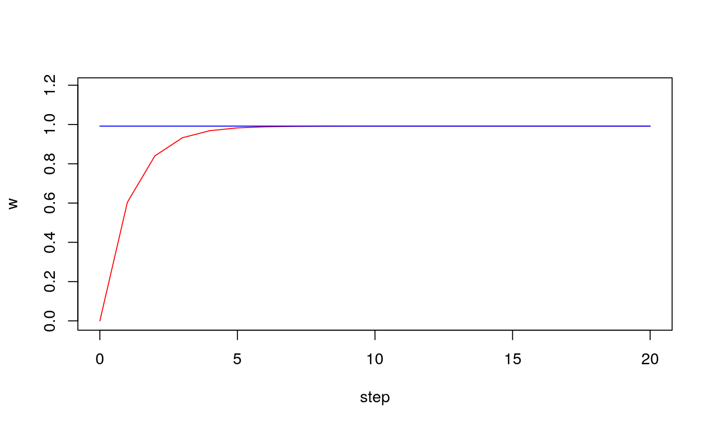
If step is too small…
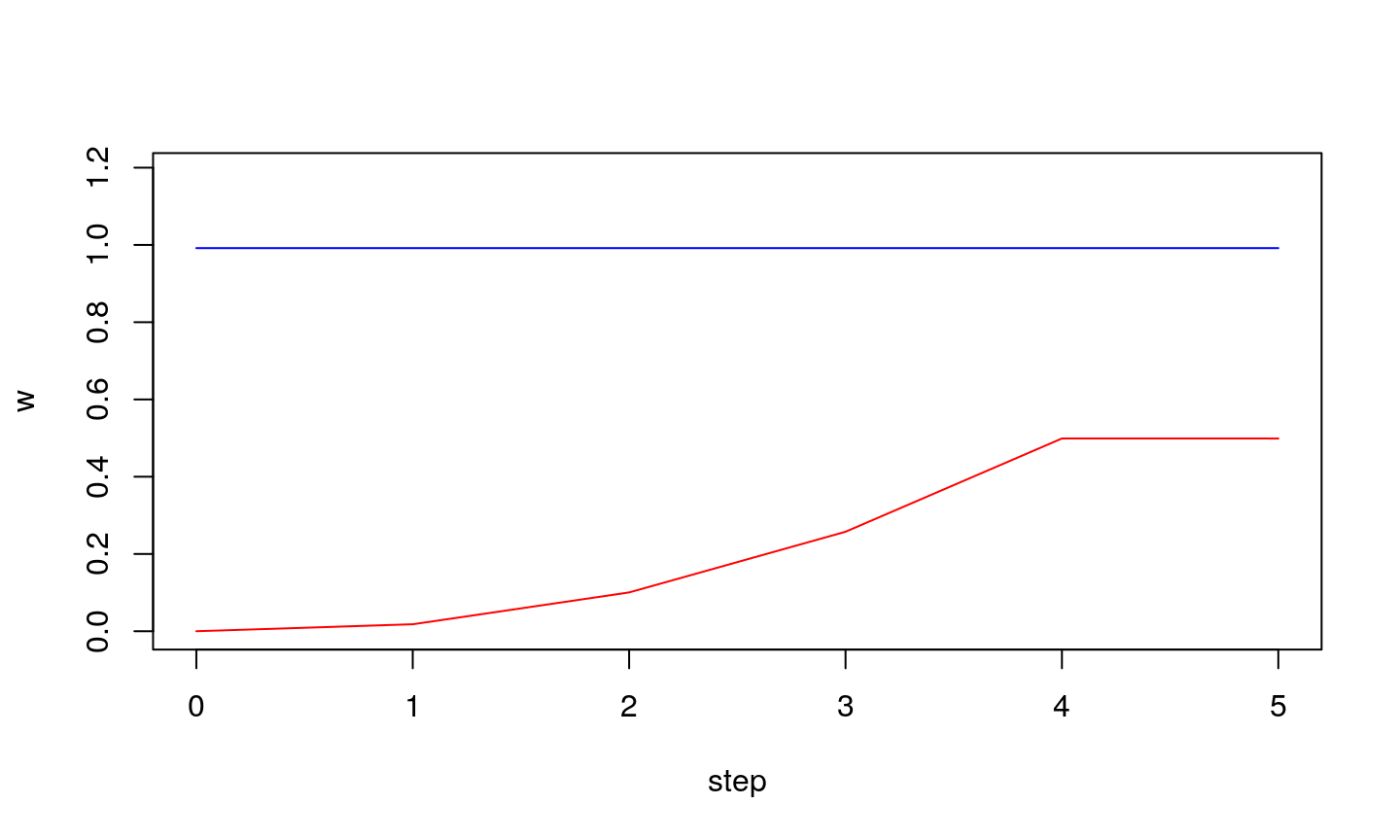
… the wights might not converge to true value
If step is large…
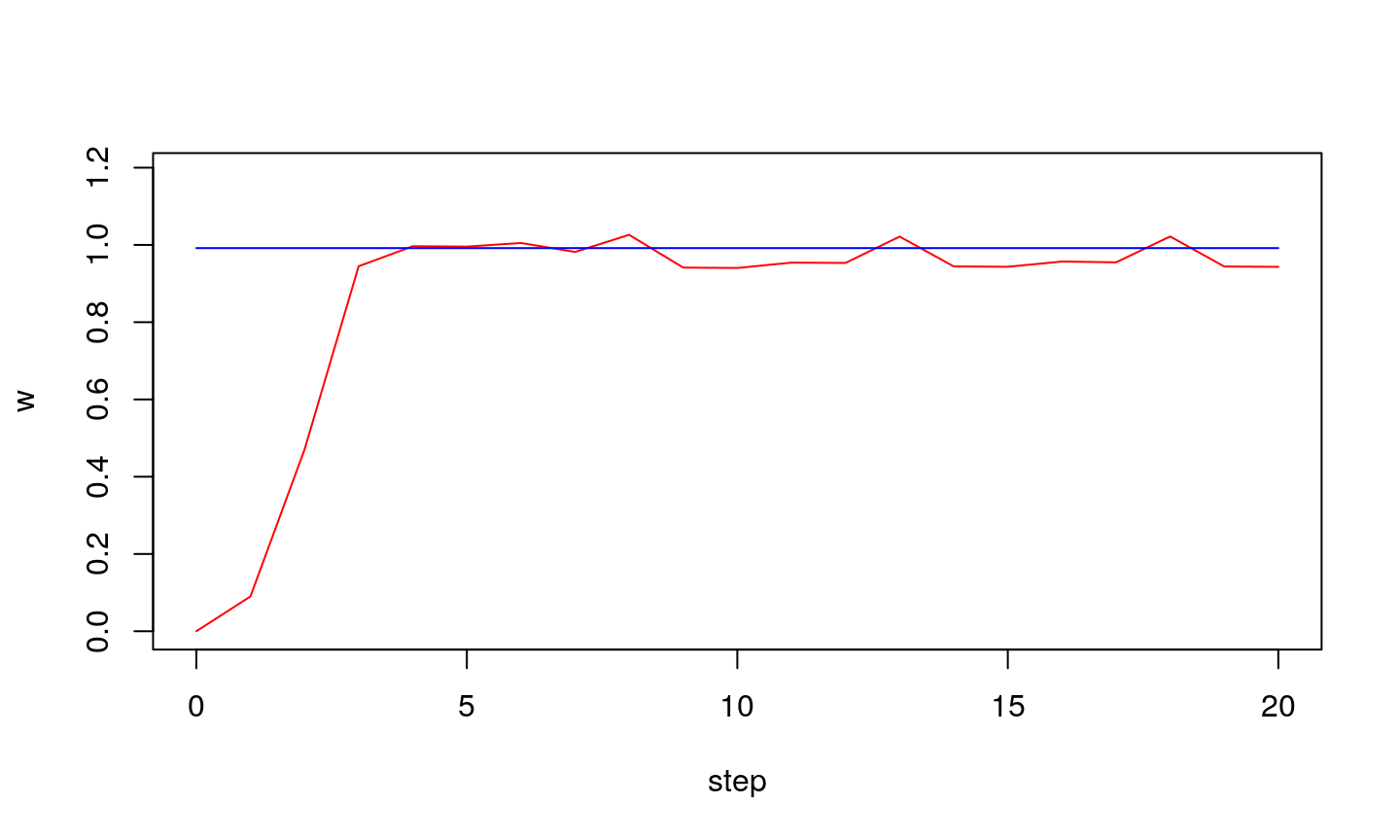
…we might get stable oscillations around optimal value.
…oscillations can also be unstable
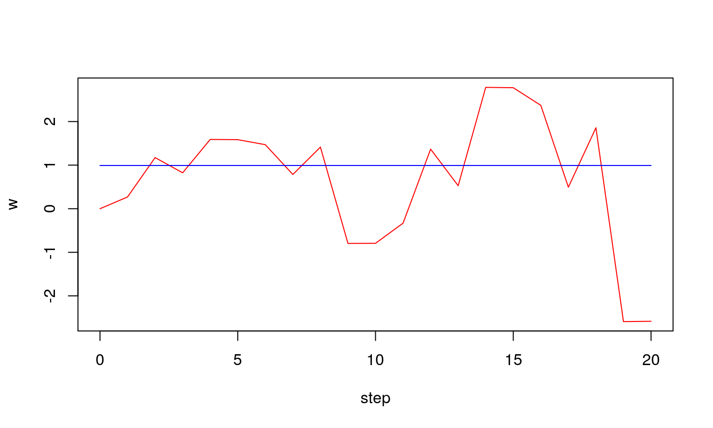
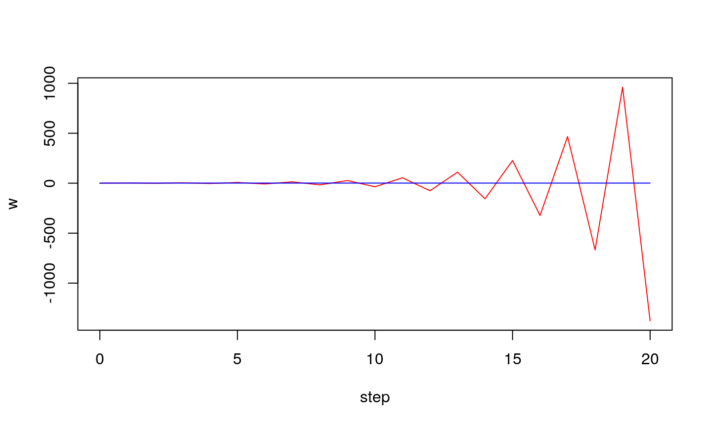
Conclusion
Learning step (\(\eta\)) is an important parameter of LMS algorithm:
- if it is too small the algorithm might not reach optimu
- if it is too large the oscillation might occur (algorithm does not converge)
Notice, the stability of the algorithm is not related to gradient approximation, but to the adaptation method (gradient descent)
Various gradient descent methods exist each with its own strength and weaknesses.
Note
- Physical analogy
- Local minimum
- Some extension of the algorithm
Physical analogy
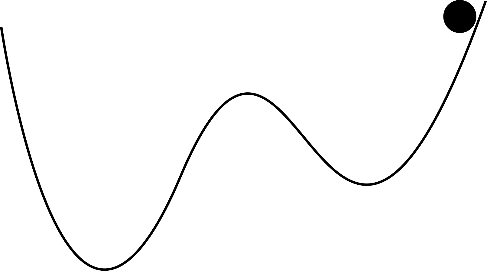
Physical analogy - a ball dropped on a surface.
Let’s propose an extension…
To reduce the probability of finding a local minimum (instead of global one), one might modify the gradient descent by introducing the inertia term (physical analogy):
\[ w(k+1) = w(k) - \eta \cdot \varepsilon(k) \cdot x(k) + \gamma \cdot \Delta w(k),\]
where \(\gamma\) is an inertion term, a \(\Delta w\) is passed from the previous step:
\[ \Delta w(k) = w(k) - w(k-1). \]
Combining neurons
- shortcomings of one neuron
- classification problem
- backpropagation
Shortcomings of one neuron
ADALINE example showed that:
- it is quite simple
- id does not do much
Actually, all one perceptron does is that it fits a curve to a given set of points. A regression analysis (i.e. a matrix calculation) could do that. And better (no optimization/convergence problem).
We use it to optimize wights as if we are solving a regression problem. Other typical case is a classification problem.
In this problem one tries to find a straight line (or more generally a curve) that divides a plain in two parts. Initial criticism of NN aimed in this direction as it was trivial to show that a single neuron cannot implement a function simple as XOR.
True, one neuron cannot solve this apparently simple problem, but two of them already can.
As we will see, true strength is not in their complexity, but in the number of neurons - although tone may increase the complexity by tampering with the network layers and neuron connectivity or with their activation function.
Linear separability
To understand why a single neuron cannot solve XOR problem we will introduce the notion of linear separability.
In the classification problem we distinguish between linearly separable and linearly unseparable classes depending on weather we can separate the classes with one straight line.
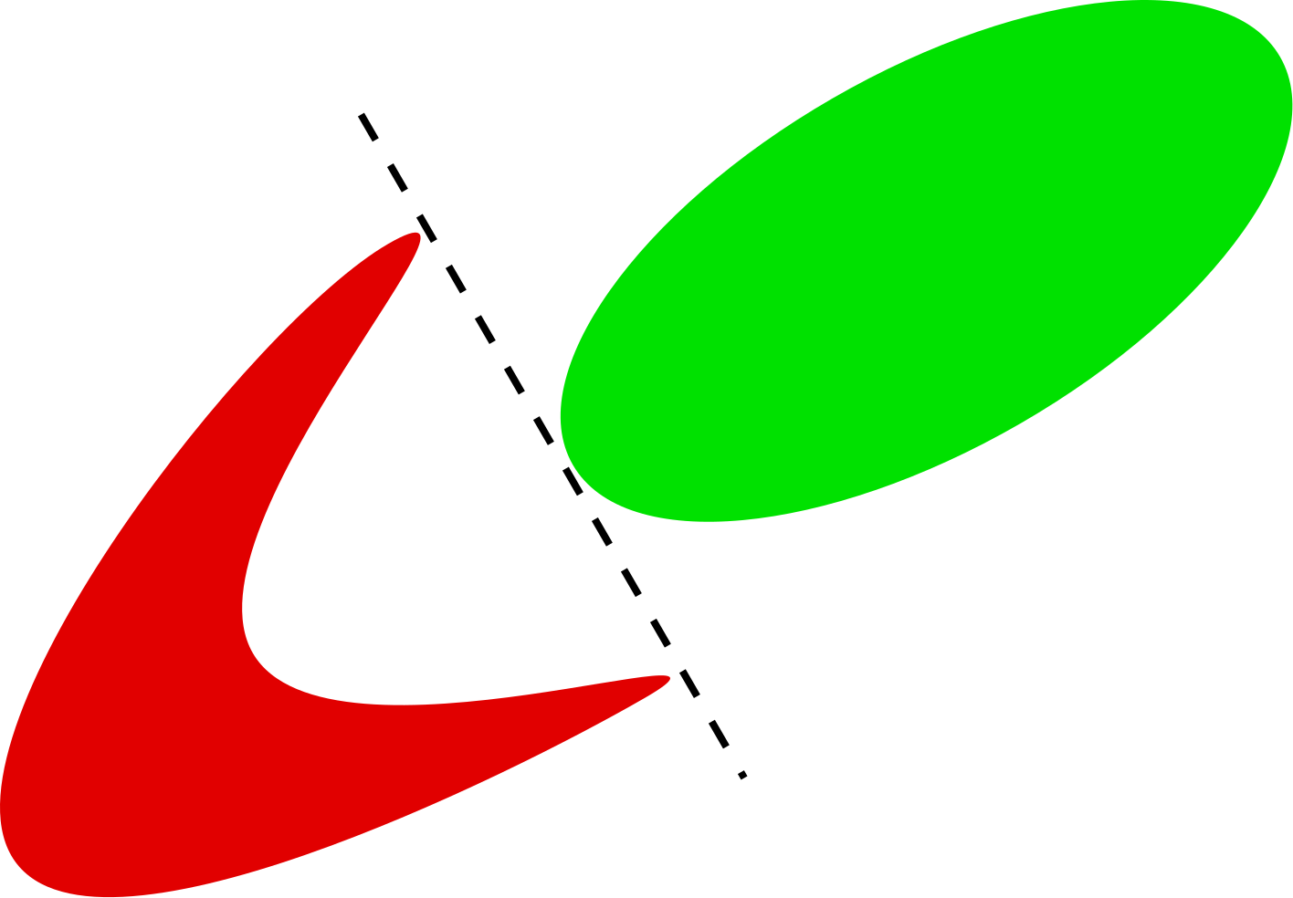
Linearly separable classification problem.

Linearly unseparable classification problem.
NN aplications
The complexity of a problem which a neural network can solve increases with the complexity of its topology.
As not many problems are linearly separable, we usually use more neurons to solve certain problems.
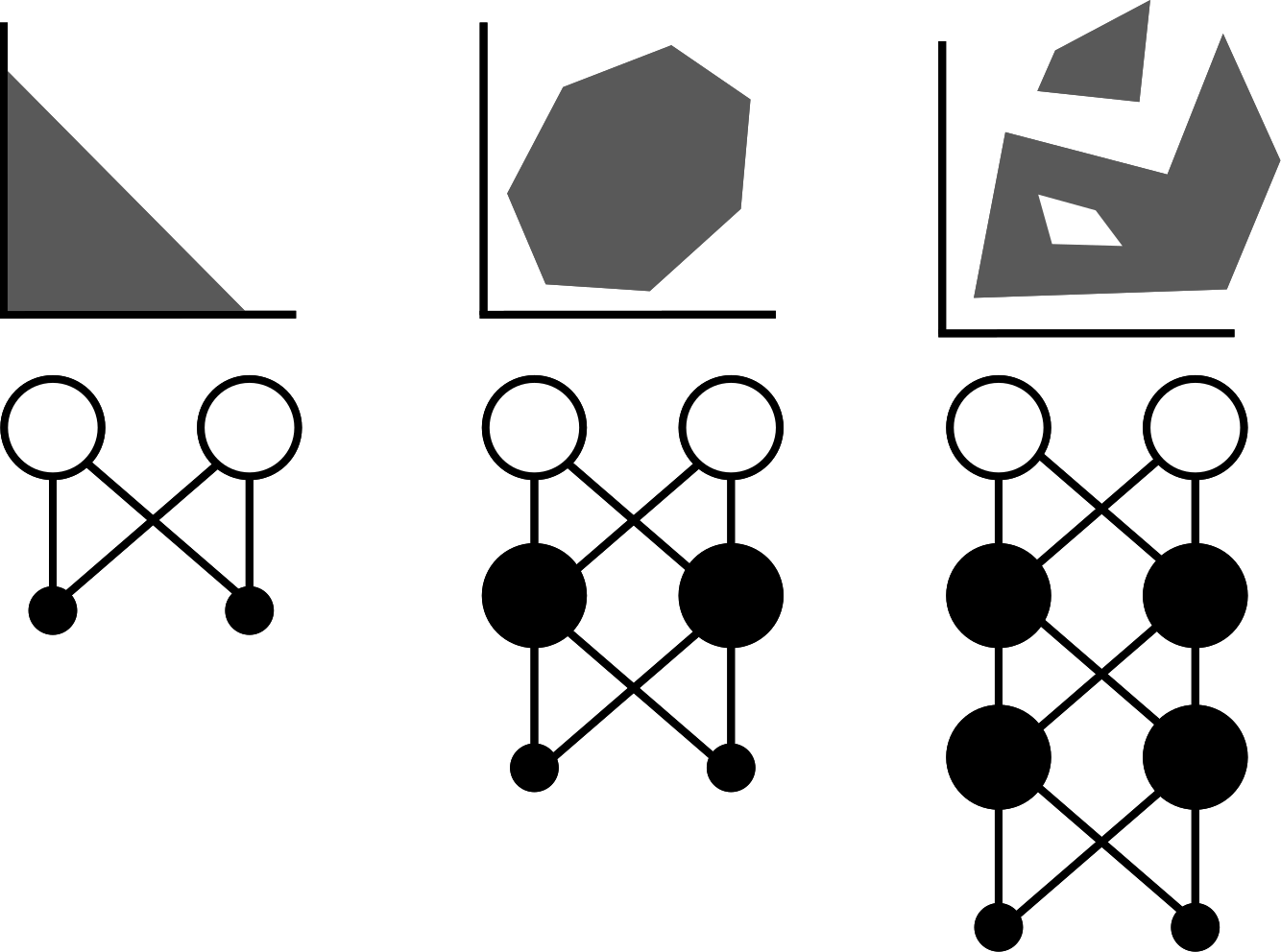
An illustration how more complex network solves more complex classification prblems.
Backpropagation
With the increase of the number of neurons we reach to the point where it is not trivial to decide the responsibility of each neuron in the final solution.
Notice that \(\Delta w\) of the solution the final layer should split to \(\Delta w\)’s of previous layer etc.
The algorithm that solves this problem is referred to as the backpropagation algorithm.
NN example
- multilayer
- hidden layer(s)
- an example on Iris dataset
NN with two neurons in hidden layer

NN with three neurons in hidden layer
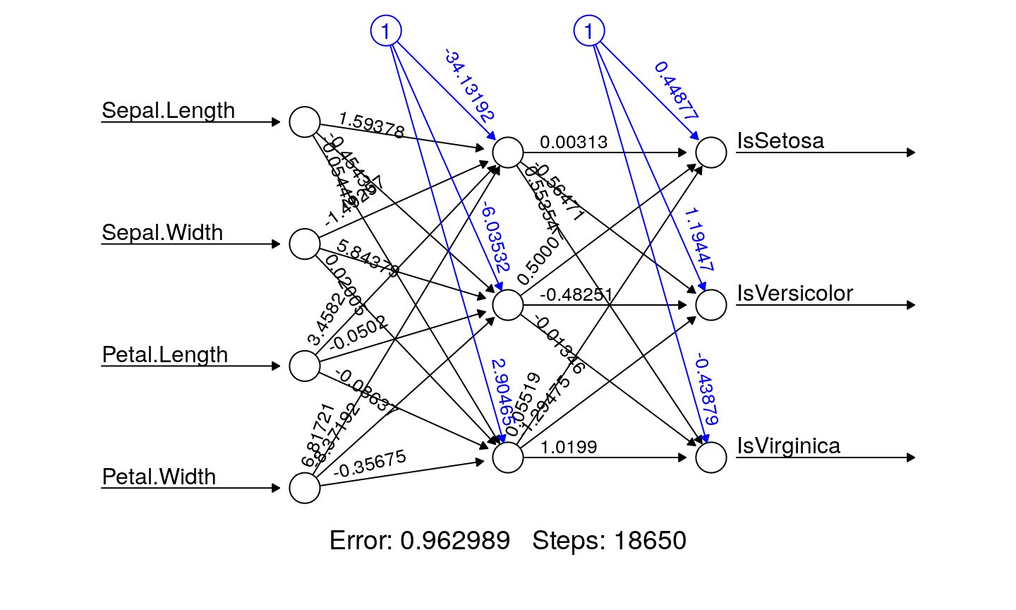
Confusion matrix
##
##               1  2  3
##   setosa     25  0  0
##   versicolor  0 24  1
##   virginica   0  3 22
Takeaways
- Why do we use learning algorithms?
- Stability problem and local minimum
- Linear separability and number of neurons
- Backpropagation